Being a data scientist (yup, that what we are called nowadays, apparently we are all the rage) and looking for my first bike to buy made me think (a lot) about what ride wanted.
Hundreds of pages on various forums talking about which bike is good, which one is better, reliability, position, torque, sound, etc etc. Yet in the end, once you have set your mind on one or two models, you still have dozens (if not hundreds) of classifieds for these models, and it is sometime hard to know whether the price is fair, a good deal, or an overpriced deal.
So, having lots of time on my hands at the moment, I started taking a quantitative approach.
- Step 1 : Get all the data (or as much as I can).
- Step 2 : Analysis, model
- Step 3 : Profit (now that I have a model, I can know whether any ad is a good deal or not).
Step 1 : Get all the data
The basis of my data is a request on a reputable motorbike classifieds website, looking for bikes which cost more than £500 (to avoid all the “wanted”) posts, and with more than 200cc. I’m not claiming the data is perfect, far from it, but if you know a better source, let me know.
Step 2 : Analysis
libs=c('data.table','knitr','ggplot2','stringr','pander','dplyr','lubridate')
invisible(lapply(libs, require, character.only=TRUE))

theme_set(theme_bw())
data = fread('~/Dev/autoray/out.csv')

data = within(data, {
  cc = as.integer(cc)
  cc[cc > 4000] = NA
  seller_type = as.factor(seller_type)
  category = as.factor(category)
  year = as.integer(year)
  year[year > 2016 | year < 1915] = NA
  mileage = as.integer(mileage)
  age = 2016 - year
  title = str_to_lower(title)
  description = str_to_lower(description)
  search = paste(title, ' ', description)
  abs = str_detect(search, 'abs')
  panniers = str_detect(search, 'panniers')
  ad_age = as.integer(Sys.time() - parse_date_time(str_extract(url, "20\\d{6}"), 'Ymd'))
  ad_age[ad_age > 365*2] = NA # Let's ignore all ads older than 2 years for ad_age
})
As you can see below, I gathered prices and information for 17043 bikes. Let’s have a look at our data :
summary(data[,sapply(data, is.numeric), with=FALSE])## price distance year mileage
## Min. : 500 Min. : 1.0 Min. :1926 Min. : 1
## 1st Qu.: 4137 1st Qu.: 54.0 1st Qu.:2008 1st Qu.: 2000
## Median : 6000 Median :114.0 Median :2012 Median : 7266
## Mean : 6857 Mean :116.7 Mean :2010 Mean : 10844
## 3rd Qu.: 8695 3rd Qu.:168.0 3rd Qu.:2015 3rd Qu.: 15900
## Max. :55950 Max. :445.0 Max. :2016 Max. :333902
## NA's :521 NA's :1832
## cc ad_age age
## Min. : 191.0 Min. : 3.00 Min. : 0.000
## 1st Qu.: 650.0 1st Qu.: 33.75 1st Qu.: 1.000
## Median : 900.0 Median : 99.00 Median : 4.000
## Mean : 921.3 Mean :133.55 Mean : 5.573
## 3rd Qu.:1170.0 3rd Qu.:182.00 3rd Qu.: 8.000
## Max. :3072.0 Max. :730.00 Max. :90.000
## NA's :19 NA's :2011 NA's :521summary(data[,!sapply(data, is.numeric), with=FALSE])## title brand seller_type category
## Length:17043 Length:17043 Private seller: 558 :16950
## Class :character Class :character Trade seller :16485 C: 57
## Mode :character Mode :character D: 36
##
## url description panniers abs
## Length:17043 Length:17043 Mode :logical Mode :logical
## Class :character Class :character FALSE:16123 FALSE:13347
## Mode :character Mode :character TRUE :920 TRUE :3696
## NA's :0 NA's :0
## search
## Length:17043
## Class :character
## Mode :character
##Here are the factors I managed to get to explain the prices.
- cc: The engine size, in cc
- seller_type : Whether the ad was posted by a private or a trade seller
- category : Whether the bike is in an insurance category (that is, a totaled bike).
- year : Year of registration of the bike
- mileage : Mileage, duh
- title, description, search : Plain text about the bike, used to add some other factors or infer the brand, model, etc.
- abs, panniers : I look for these words in the titles, description. Not perfect, especially because I look them as strings, not as words. So a description about an absolute steal would match an abs. Yeah, that sucks, but I haven’t had the time to research what NLP tools R offers for stemming.
- ad_age : The age of the ad, calculated from a time stamp in the url. This one actually gets lots of
N/A, because some urls are for ads and don’t show the timestamp.
Step 2 : Analysis
Impact of the age on the price
ggplot(data) + geom_smooth(aes(y=price, x=age, color=category)) + scale_x_continuous(breaks = seq(0,90,10))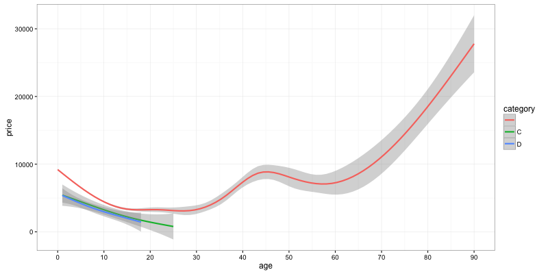
What can we see on this graph ?
- Prices go down almost linearly during the first 15 years.
- After that, you can expect prices to remain kind-of stable for bikes which are just about to become vintage.
- Motorbikes more than 30 years old start to see a constant rise in value.
- Cat C and Cat D bikes have a value that is constantly lower than the value of non-category motorbikes. They decrease in value steadily.
Now, let’s focus on bikes which are less than 15 years old, not in a category.
data = subset(data, age <= 15 & category == "")We can evaluate this discount :
summary(lm(price ~ age, data))##
## Call:
## lm(formula = price ~ age, data = data)
##
## Residuals:
## Min 1Q Median 3Q Max
## -8461 -2020 -479 1308 47431
##
## Coefficients:
## Estimate Std. Error t value Pr(>|t|)
## (Intercept) 8961.18 40.13 223.28 <2e-16 ***
## age -442.60 6.81 -64.99 <2e-16 ***
## ---
## Signif. codes: 0 '***' 0.001 '**' 0.01 '*' 0.05 '.' 0.1 ' ' 1
##
## Residual standard error: 3236 on 15503 degrees of freedom
## Multiple R-squared: 0.2141, Adjusted R-squared: 0.2141
## F-statistic: 4224 on 1 and 15503 DF, p-value: < 2.2e-16We see whe should expect a loss of value of £442/year, but it makes more sense to assume this loss in value should be a percentage of the original value, which would be 442/8961, or about 5%/year for the first 15 years.
Impact of brands
As a first approximation, we can take the first word of the ad title to get the brand. Brands that use several words will be trimmed, but that should be good enough for now.
data$brand = as.factor(word(data$title))
brands = data %>% group_by(brand) %>% tally(sort = TRUE)
big_brands = brands[1:8]$brand
data$big_brand = data$brand %in% big_brands

# Let's try a colorblind friendly version
cbPalette <- c("#999999", "#E69F00", "#56B4E9", "#009E73", "#F0E442", "#0072B2", "#D55E00", "#CC79A7")
ggplot(data[data$big_brand]) + geom_smooth(aes(y=price, x=age, color=brand), se = FALSE) + scale_colour_manual(values=cbPalette)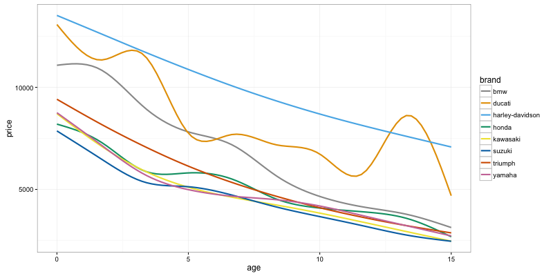
Here we can see not only the difference in average price between brands (be careful, I haven’t distinguished between models here), but also how these decay with time.
We can see that Harleys are consistently more expensive, but seem to hold their value relative to other bikes quite well. Ducatis see a sharp drop at around 5 years. BMW are more expensive than the other brands as well in their first 7 years or so, but then drop in price to be actually cheaper than other brands. My guess is that because they are more expensive, they tend to be favoured by people able to buy them new, but the second-hand market for them isn’t that great.
Engine size
ggplot(data) + geom_smooth(aes(y=price, x=cc))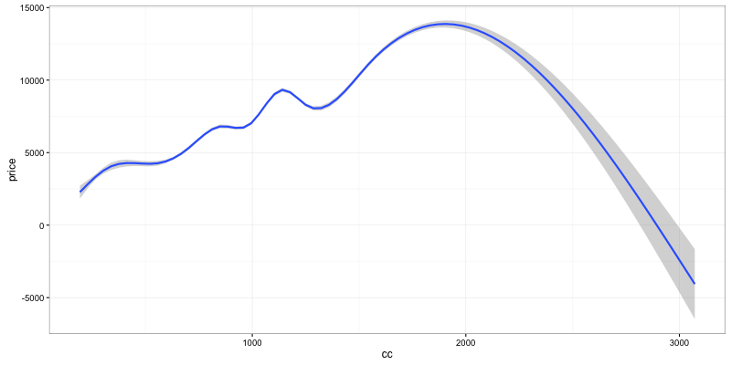
Not much to see here by default, we can just see that the price of a bike grows (almost linearly) with the engine size. That is until 1800cc (Goldwings), then beyond 2000cc you enter the realm of the Rocket III which is just less expensive than the goldwing.
Mileage
Some bikes seem to have crazy mileage (300k), so let’s stick to stuff with reasonable values, less than 100k.
ggplot(subset(data, mileage < 100000)) + geom_smooth(aes(y=price, x=mileage))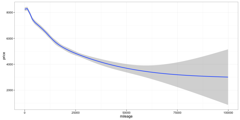
Big surprise, the price drops as the mileage increase. The effect seems almost linear to start with, then seems to decay. We can probably work with a linear decay for the first 25k, beyond that it just makes sense to use a log decay…
summary(lm(price ~ mileage, subset(data, mileage < 25000)))##
## Call:
## lm(formula = price ~ mileage, data = subset(data, mileage < 25000))
##
## Residuals:
## Min 1Q Median 3Q Max
## -7708 -2237 -612 1667 47778
##
## Coefficients:
## Estimate Std. Error t value Pr(>|t|)
## (Intercept) 8.208e+03 4.409e+01 186.18 <2e-16 ***
## mileage -1.569e-01 4.401e-03 -35.65 <2e-16 ***
## ---
## Signif. codes: 0 '***' 0.001 '**' 0.01 '*' 0.05 '.' 0.1 ' ' 1
##
## Residual standard error: 3349 on 12764 degrees of freedom
## Multiple R-squared: 0.09055, Adjusted R-squared: 0.09048
## F-statistic: 1271 on 1 and 12764 DF, p-value: < 2.2e-16summary(lm(price ~ log(1 + mileage), data))##
## Call:
## lm(formula = price ~ log(1 + mileage), data = data)
##
## Residuals:
## Min 1Q Median 3Q Max
## -8961 -2347 -603 1613 48229
##
## Coefficients:
## Estimate Std. Error t value Pr(>|t|)
## (Intercept) 9715.54 91.98 105.6 <2e-16 ***
## log(1 + mileage) -366.54 10.97 -33.4 <2e-16 ***
## ---
## Signif. codes: 0 '***' 0.001 '**' 0.01 '*' 0.05 '.' 0.1 ' ' 1
##
## Residual standard error: 3370 on 14061 degrees of freedom
## (1442 observations deleted due to missingness)
## Multiple R-squared: 0.0735, Adjusted R-squared: 0.07344
## F-statistic: 1115 on 1 and 14061 DF, p-value: < 2.2e-16What we can see here is that the price of the bike seems to drop by 0.1569 per mile, or £156/1000miles. Translating again to a percentage of the intercept, we get 0.0190058 or about 1.9% per 1000 miles.
This figure could depend on the brand quite heavily (and more importantly on the type/model) of bike. You’d expect tourers, VFRs and R1200RT to hold their value with mileage a lot better than some shiny supersport bikes. We’ll have a look at that in another post.
Mileage + age
Mileage and age are obviously very (read 0.6531262 = 65%) correlated, so we’ll have to use both in our price regression.
summary(lm(price ~ age * log(1+mileage), subset(data, mileage < 100000)))##
## Call:
## lm(formula = price ~ age * log(1 + mileage), data = subset(data,
## mileage < 1e+05))
##
## Residuals:
## Min 1Q Median 3Q Max
## -7869 -1921 -400 1292 47533
##
## Coefficients:
## Estimate Std. Error t value Pr(>|t|)
## (Intercept) 8325.324 98.211 84.770 < 2e-16 ***
## age -3.961 45.923 -0.086 0.931
## log(1 + mileage) 62.846 13.223 4.753 2.02e-06 ***
## age:log(1 + mileage) -45.364 4.654 -9.748 < 2e-16 ***
## ---
## Signif. codes: 0 '***' 0.001 '**' 0.01 '*' 0.05 '.' 0.1 ' ' 1
##
## Residual standard error: 3075 on 14055 degrees of freedom
## Multiple R-squared: 0.2289, Adjusted R-squared: 0.2287
## F-statistic: 1390 on 3 and 14055 DF, p-value: < 2.2e-16We can pretty much ignore the coef in front of age (low tstat), we get something that is roughly : $ price = 8325 + logMileage * (62 - 45 * age) $
Are private seller cheaper than trade sellers ?
ggplot(data) + geom_smooth(aes(y=price, x=age, color=seller_type)) + scale_x_continuous(breaks = seq(0,90,10))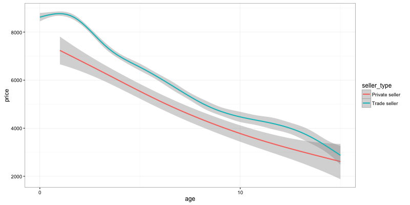
The answer seems consistently yes !
Do good deals go quickly ?
It seems intuitive to think that good deals will be sold quickly, and the longer an ad has been there, the more likely it is that the bike is above its market price. Trade sellers and their automated posting software would skew the results, by having software that refreshes ads every-so-often, but we should still see some effect.
ggplot(data) + geom_smooth(aes(y=price, x=ad_age)) + scale_x_continuous(breaks = seq(0,365*2,30))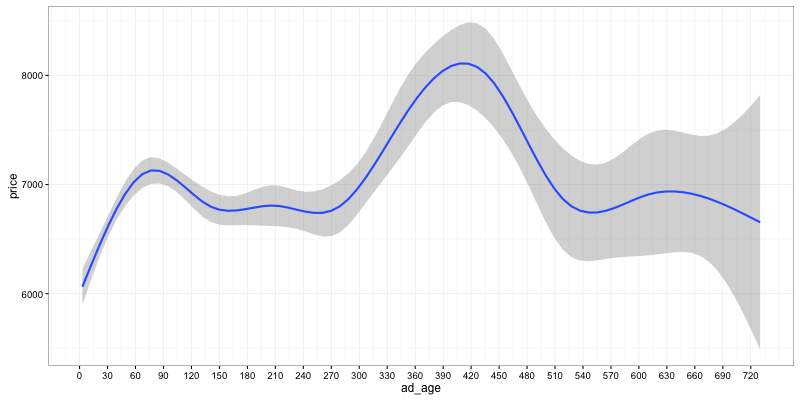
So yes, our intuition holds, it looks like the average price for new ads is around £1000 less than for ads that are 2 months old. There is a bias here, because many ads for new models are put by dealers and left forever. Let’s run the query again, this time only looking a bikes which are more than 2 years old, and comparing dealers/private sellers.
ggplot(data[age >= 2]) + geom_smooth(aes(y=price, x=ad_age, color=seller_type)) + scale_x_continuous(breaks = seq(0,365*2,30))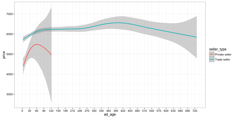
What we can see here is still that good deals move quickly, and this difference is even more pronounced for private sellers than it is for dealers. An ad that has been out for two months is on average £1000 more expensive than the one that will get sold within its first few days.
We’ll see in a next post whether it still holds when looking at data for one single model.
ABS
ggplot(data) + geom_smooth(aes(y=price, x=age, color=abs)) + scale_x_continuous(breaks = seq(0,90,10))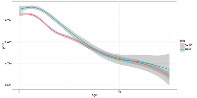
Well, we can see that ABS definitely seems to keep its increased price, at least for recent bikes. One has to be careful though, because ABS is usually found on higher end bikes, so this difference in price could just be a bias. One would have to do a price comparison for a specific model (with enough data).
Distance to london
ggplot(data) + geom_smooth(aes(y=price, x=distance))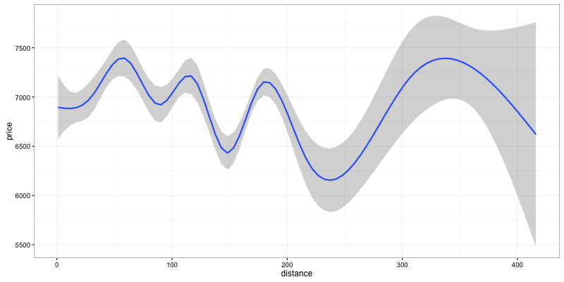
Hard to say anything here. Could be some bias from big cities that appear at some distance from London. Given we don’t have the postcode for all ads, it’s hard to go beyond this useless graph.
Conclusion
I’ve only looked at a few things, and it seems obvious here that many results are probably biased given I’m not filtering to a specific model.
Next time, I’ll look at the most frequent bike of the most frequent brand, and we’ll see if these results still hold. Plus yeah, we’ll have a first look at our pricing model and try to find some underpriced bikes.
Stay tuned (and feel free to guess what model we’ll be looking at in the comments, or let me know if you’d be interested in another specific analysis).
If you want to re-publish all or part of this data/graphs/article, get in touch. Just ask.
I’d like to get some data on insurance as well, but it’s a lot harder to gather. If you know a way, let me know…
Edit 1 : 2015-02-04 11:24 GMT - Changed the brand graph to only use 8 brands but with colorblinds-friendly palette.